Our Hope

Before we begin, we need to establish what large language models (LLMs) are. LLMs are a type of artificial intelligence model trained on large amounts of text to understand and generate human-like language. In particular, they do one task really well: predicting the next word in a sequence. With that in mind, let's develop a model that does exactly that.

Suppose we give our model the phrase "once upon a". We want it to predict the next word: "time". More generally, we want the model to predict the next word given all previous words in the sequence. To simplify the problem conceptually, let's think of each word as being associated with some information. The information associated with a word may be influenced by earlier words but it is the information for the last word that is used to predict the next one. In our example, the information associated with "a" is used to predict the next word, "time". Similarly, the information for "upon" should help predict "a", and that for "once" should help predict "upon".

We will represent this notion of information with a vector, which we'll call a context vector. Our goal is to predict the next word given the current word's context vector. How do we do this? It turns out that this is just multiclass classification, where the classes are all the words in our vocabulary.

To do this, we can learn a weight matrix that transforms the context vector into a set of scores — one for each word in the vocabulary. More specifically, we compute the dot product between the context vector and each row of this matrix. Since there's a row for every word in the vocabulary, we get a score indicating how likely the model thinks each word is to come next. Then, we select the word with the highest score as the model's prediction of the next word.

We would hope that the dot product between the context vector for "a" (which we will call $\vec{x}_\text{a}$) and the row in the weight matrix corresponding to the word "time" is the highest. That is, we would hope that the context vector for "a" is most similar to that row.

We can now see that the problem has reduced to making the context vector for "a" and the row corresponding to "time" as similar as possible.

An Initial Idea

Our first idea may be to represent "a" with some fixed vector. We will call this the embedding of "a". Then, we learn the matrix weights so that the row for “time” becomes as similar as possible to the embedding of “a”. There is an issue with this approach though: we only look at the word "a" to determine the next word. So if we were able to train the model to output "time" given the embedding of "a", it would correctly complete the phrase "once upon a time", but it would incorrectly complete a phrase like "the sun is a star" and instead output "the sun is a time".

We would like to consider all the words that came before it. So instead of using just the embedding of "a", we could define its context vector as the average of the embeddings of "once", "upon", and "a". That way, when we feed the context vector into our classifier, it has baked in information about all preceding words.

This is a lot better. It solves our "the sun is a time" problem. But it raises another issue. Take the phrase "the capital of France is" which we train to complete with "Paris". That means we've learned the matrix so that the context vector for "is" — the average of the embeddings of "the", "capital", "of", "France", and "is" — is most similar to the row for "Paris".

Now consider the phrase "the capital of Spain is". All words except one are the same, so the average embedding vector will be nearly identical to the one for the France sentence. Hence, it is likely that our classifier will output "Paris" here as well. So, we'd get "the capital of Spain is Paris" instead of the desired "the capital of Spain is Madrid".

So what went wrong? The issue is that all words were weighted equally. We would like to weigh certain words more than others. In the example above, we would like to weigh the words "France" and "Spain" more in their respective phrases. But how do we decide how much to weigh each word? To develop an answer to that question, it will help to get visual.

Embeddings

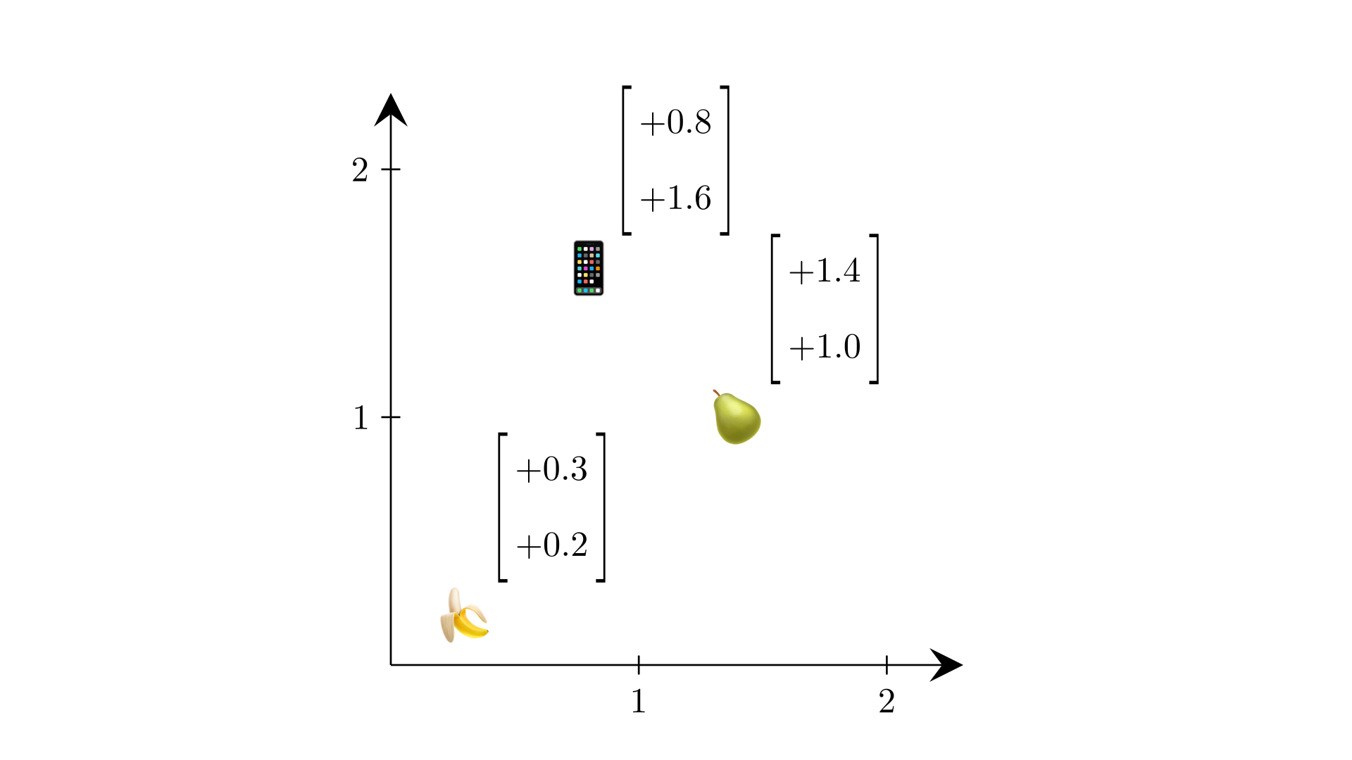
Earlier, we said that we would represent "a" with a fixed vector — that we would embed it. But what exactly does that mean? We want to associate each word in our vocabulary with a list of numbers. For now, we will say a list of two numbers. But how should we assign numbers to words? To start, we could just assign each word two random numbers. Take the words "banana", "pear", and "phone". We may randomly assign them the numbers $[+0.3, +0.2]$, $[+1.4, +1.0]$, and $[+0.8, +1.6]$. We can plot these in a 2D space.

We can plot our random embeddings in a 2D space.

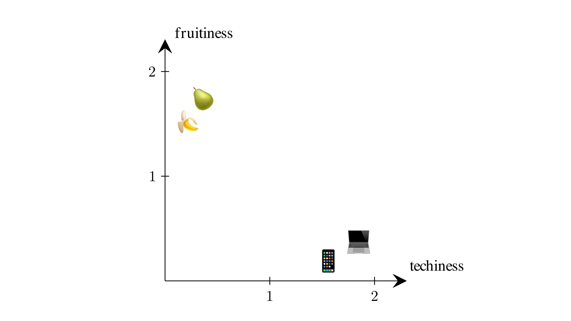
Let's consider whether we can do something more meaningful. A property we might hope to have is that similar words have similar embeddings and very different words have very different embeddings. Why? As we've seen, very similar inputs to our classifier tend to produce the same or very similar outputs. So we want words that are likely to be followed by the same next word to have similar embeddings, and words that are unlikely to share the same next word to have very different embeddings.

In our "banana", "pear", and "phone" example, we would like "banana" and "pear" to have similar embeddings — that is be near each other in 2D space — because they are both fruits, and "phone" to have a very different embedding. To make sense of this distinction, we can assign the idea of fruitiness to one of the axes and the idea of techiness to the other axis.

A more meaningful embedding where similar words are near each other.

Words Pulling Words

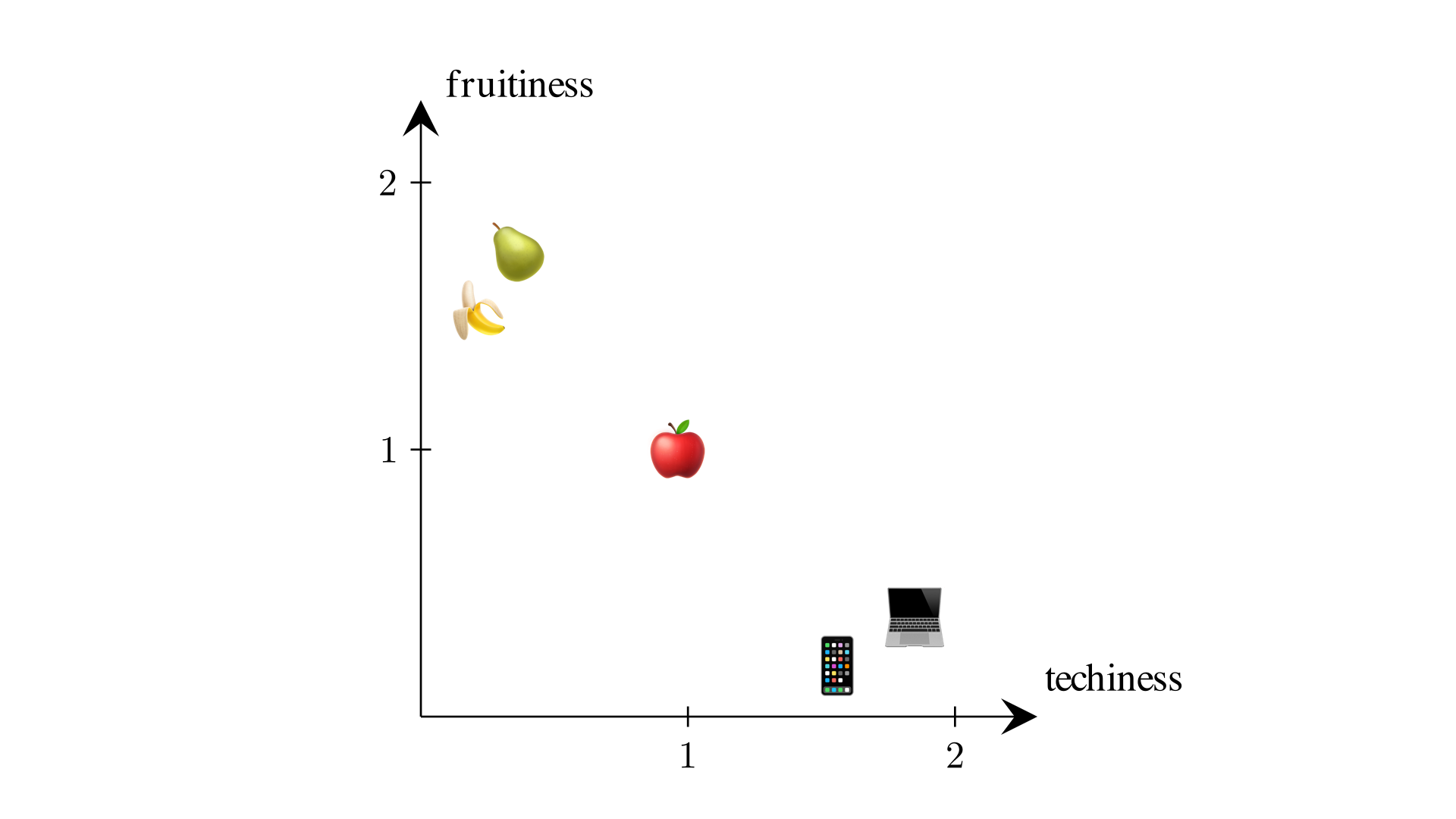
Let's now think about where to place the word "apple". Where should we put it? It depends on how "apple" is used. If it appears in the phrase "I ate a banana and an apple", it should go near the fruits, but if it is in the phrase "I got a new phone from apple", it should be by the technology devices. So there is no one great choice for the embedding of "apple". The best we can do is place it somewhere between the two. That's what we will do in our generic embedding.

Generic embedding of "apple".

When we are given the phrase it appears in, we would like to adjust the embedding of "apple" to better represent how the word is used in that phrase. In the first example we would like to move "apple" closer to the fruits, and in the second closer to the technology devices.

How do we know where we want to move it? Some of the other words in the phrases give very good clues about what meaning of "apple" is intended. In "I ate a banana and an apple", the word "banana" tells us that it is talking about the fruit. And in "I got a new phone from apple", the word "phone" indicates that it meant the technology brand.

Returning to the embedding space, we want "banana" to pull "apple" closer to it. And in the second example, we want "phone" to pull "apple" closer to it.

What about the other words in the phrase? How do we know that "banana" is the word that should pull "apple" and not any of the other words? Let's plot the embeddings of the other words. We can see that they are not very close to "apple" because they are not very similar to "apple". The words that are most similar to "apple" pull it the most. So, all words exert some amount of pulling force, but the effect is dominated by the most similar words. I like to compare this to gravity (where the objects have the same mass). Objects that are closer exert more gravitational force on each other than objects that are farther away.

Let's now think about how to determine where exactly to move "apple" — that is how much each word pulls "apple". We start by computing the similarity between "apple" and every word. We will use the dot product as our measure of similarity. Two vectors have a very high dot product if they point in similar directions and have similar lengths, and a very low dot product if they point in opposite directions.

As we would expect, other than "apple" and "apple", "apple" and "banana" have the highest dot product, so they are most similar.

We want to use these dot products to determine how much we should nudge "apple" in the direction of each word. At an extreme, where we want "apple" to move completely to "banana", we would simply set 100% of the new "apple" vector to the coordinates of the "banana" vector. We can write this as the following linear combination:

What series of dot products would suggest this linear combination? One dot product should be incredibly large (the one between "apple" and "banana") and the rest should be incredibly small.

If we instead want "banana" to pull "apple" halfway between it and the original position for "apple", we would want this linear combination:

We want this if the dot products between "apple" and "apple", and "apple" and "banana" are large and pretty equal, and the rest are very small in comparison. If instead all the dot products are pretty similar, meaning that "apple" is equally similar to all words, we would want all words to pull "apple" equally. So we'd want a linear combination like this:

We see that we want all coefficients to be between 0 and 1, and for them to sum to 1. We also want to emphasize the larger dot products. Those are the most similar words, so we want them to pull more. A function that accomplishes this is the exponential function $f(x) = e^x$. So, we will exponentiate each dot product. In order for the coefficients to sum to 1, we divide each term by the sum of all the terms. This is called normalization. The function we have described is referred to as softmax and is usually written like this:

These coefficients are referred to as attention scores. They tell us how much to pay attention to each word — that is how much each word should pull "apple". We can now compute the linear combination to get the updated vector for "apple".

The process we have just developed is called attention. Specifically, it is one iteration of attention. We can repeat this process multiple times to further refine the vector for "apple".

Attention is a Weighted Average

Let's return to our original goal: predicting the next word in a sequence. To do this, we feed the context vector for the last word into a multiclass classifier. The classifier uses a weight matrix with one row per word in the vocabulary. For the model to output the correct word, the row corresponding to that word must be as similar as possible to the context vector.

We realized that simply using the embedding of the last word as the context vector was not ideal. It would incorrectly predict the same next word for both "once upon a" and "the sun is a" — because it's only looking at the word "a" to make the prediction.

Next, we considered defining the context vector of the last word to be the average of the embeddings of it and the words before it. This was an improvement — it solved the "the sun is a time" problem. But it still had a weakness: sequences that differ by just one or two words, like "the capital of Spain is" and "the capital of France is", would end up with very similar context vectors and, therefore, the same prediction — even when the correct next words are very different.

The takeaway was clear: not all words should be weighted equally. Some are far more relevant than others when predicting the next word. The question we didn't know how to answer was how to determine how much to weigh each word. That's exactly what attention gives us: a way to compute a weighted average of the embeddings. The idea of words "pulling" other words is realized mathematically by computing the dot product between embeddings, applying softmax, and using the resulting scores as weights. This is attention.

The result of attention, or of multiple iterations of attention, is an updated embedding vector that has soaked in the context that the word appears in. We use it as the context vector that we feed into the classifier.

And that's the basic mechanism behind large language models like ChatGPT. If you've followed along this far, you now understand the core idea at the heart of today's most powerful AI systems.

But to turn this into an "intelligent" system — one that can complete sequences with nuance and coherence — we'll need to refine the mechanism further. Let's build those improvements together.

The Whole Phrase

So far, we've only looked at how the word "apple" is pulled. That is, we've only applied attention to update the vector for "apple" based on the other words. But in practice, we want to apply attention to all words in the phrase. We want each word to be pulled to a better place for it, given the surrounding words. Why? There are two main reasons:

1. As we've alluded to, we often apply multiple iterations of attention to refine the vector for a word. Consider the phrase "I ate an orange and an apple". Here, we want "orange" to give context to "apple", but we also want "apple" to give context to "orange". We want "apple" to help "orange" understand that it’s being used as a fruit, not a color. This will ultimately benefit the context vector for "apple". When it is pulled by all the words in the phrase in the next iteration of attention, it will be pulled by the updated vector for "orange" that has more fruit characteristics than the original vector.
2. During training, we predict the next word at every position, not just the last one. So, given the phrase "I ate a banana and an apple", we ask it to predict every next word in the sequence. For example: given "I", predict "ate"; given "I ate", predict "an"; and so on. As we're making predictions at every word, we need the vector for every word to be as informative as possible.

We can visualize what we have done so far in computing attention scores for "apple" by creating a column for every word in the phrase and creating a row for "apple". We fill in the row by computing the dot product between "apple" and the word in each column. We can extend this to more words. We will add a row for each other word and repeat the same computation steps.

We now have a table of dot products which tell us how similar each word is to every other word. Using linear algebra notation, we can write this table of dot products in a compact way. If we take all embedding vectors of the words and stack them as rows in a matrix, which we will call $X$, we can compute the matrix of dot products by doing matrix multiplication of $X$ and a transposed version of $X$. That is $XX^T$.

Just as before, the next step is to apply softmax. Previously, we only did so to the "apple" row, but we now do it to every row. We often write $\text{softmax}(XX^T)$ to mean that we apply softmax to each row.

This gives us a matrix of attention scores. Finally, just as before, we use each row of attention scores to compute a weighted average of all embedding vectors — one for each word.

This can be written as $\text{softmax}(XX^T)X$. The rows of this final matrix contain the updated vectors for each word.

As a quick aside, it may not be obvious why this matrix multiplication gives us a row-wise weighted average. Let's work through a small example to see why it works. Let $A = \text{softmax}(XX^T)$ for brevity. We will denote the entry in the $i^\text{th}$ row and the $j^\text{th}$ column in $A$ as $a_{ij}$ and in $X$ as $x_{ij}$. So, we have the two matrices:

Let's first multiply $A$ and $X$:

Next, let's rewrite this as the addition of two matrices:

Now, we factor out the coefficient from each row:

Finally, let's add the two matrices back together:

The vector $[ x_{11} \;\; x_{12} ]$ is the the first row in $X$ and thus the first embedding vector $\vec{x_1}$ and $[ x_{21} \;\; x_{22} ]$ is the second embedding vector $\vec{x_2}$. We can now see that this indeed produces a row-wise weighted average.

Transforming the Embeddings

Let’s revisit the embedding space we used when introducing the idea of words pulling words. We had one cluster of fruits and another cluster of technology devices, and we used attention to move the embedding of "apple".

Our original embedding space

Were those the best embeddings for this task? The embeddings are made to be great general-purpose embeddings, but they may not be the best we can do for this very specific goal of separating the two meanings of "apple". Soon, we'll explore what a more useful embedding space might look like for this task.

But first, let's discuss how we can obtain new embeddings from our original embeddings. What we need is a function that, given a vector, outputs a different vector. Linear transformations provide a simple and powerful way to do this — they multiply a vector by a matrix to produce a new vector.

In our case with two-dimensional embedding vectors, any $2\!\times\!2$ matrix $M$ will transform the embedding vector $\vec{x}$ into a new two-dimensional vector.

When we apply a linear transformation to the entire space — that is to every vector — we also transform the coordinate system itself. What we mean by that is that we transform the vectors $[0, 1]$ and $[1, 0]$, which are known as the unit basis vectors and define the coordinate system. This makes it easy to visualize a linear transformation and to plot the transformed vectors. For example, to plot the transformed version of the vector $[1, 2]$, we place it at the point $(1, 2)$ relative to the new (transformed) axes.

A Better Space for Pulling Words

Now that we understand how linear transformations can create new embedding spaces, let's explore why that's useful. Consider three embedding spaces: the original and two transformed versions.

Is one space better than the others for pulling the word "apple"? Remember, our goal is to separate the two meanings of "apple". In space B, attention barely distinguishes the two meanings of "apple" — the vectors end up too close. But in space C, they're pulled far apart, which is exactly what we want.

Let's now use transformed vectors — instead of the original ones — when computing the linear combination that defines the new "apple" vector. The transformed vectors are referred to as values, denoted $v$, and the matrix used to compute them is denoted $W_V$.

But what about the coefficients — the attention scores that tell us how much each word should pull "apple"? Should we use these same transformed vectors to compute them too? We could — and that might already work better than using untransformed embeddings. But there's an even more powerful approach. We'll come back to that in a moment.

Asymmetric Pull

As we've discussed, attention isn't just applied to a single word like "apple" — every word pulls and is pulled by every other word. So just as "banana" pulls "apple", "apple" also pulls "banana".

The pulling force that one word exerts on another is completely determined by the similarity of the two words. This means that it is always the case that "banana" pulls "apple" just as much as "apple" pulls "banana". This symmetry is not always desirable. We can find examples where we'd want asymmetric pull.

Take the words "bride" and "ring". If a phrase contains the word "bride", it is quite likely that the word "ring" will appear. So, we want "bride" to exert a strong pulling force on "ring". On the other hand, if a phrase contains the word "ring", it is not as likely that the word "bride" will appear. It could be referring to a piece of jewelry, a boxing ring, or perhaps a phone call. So, we want "ring" to exert a weaker pulling force on "bride".

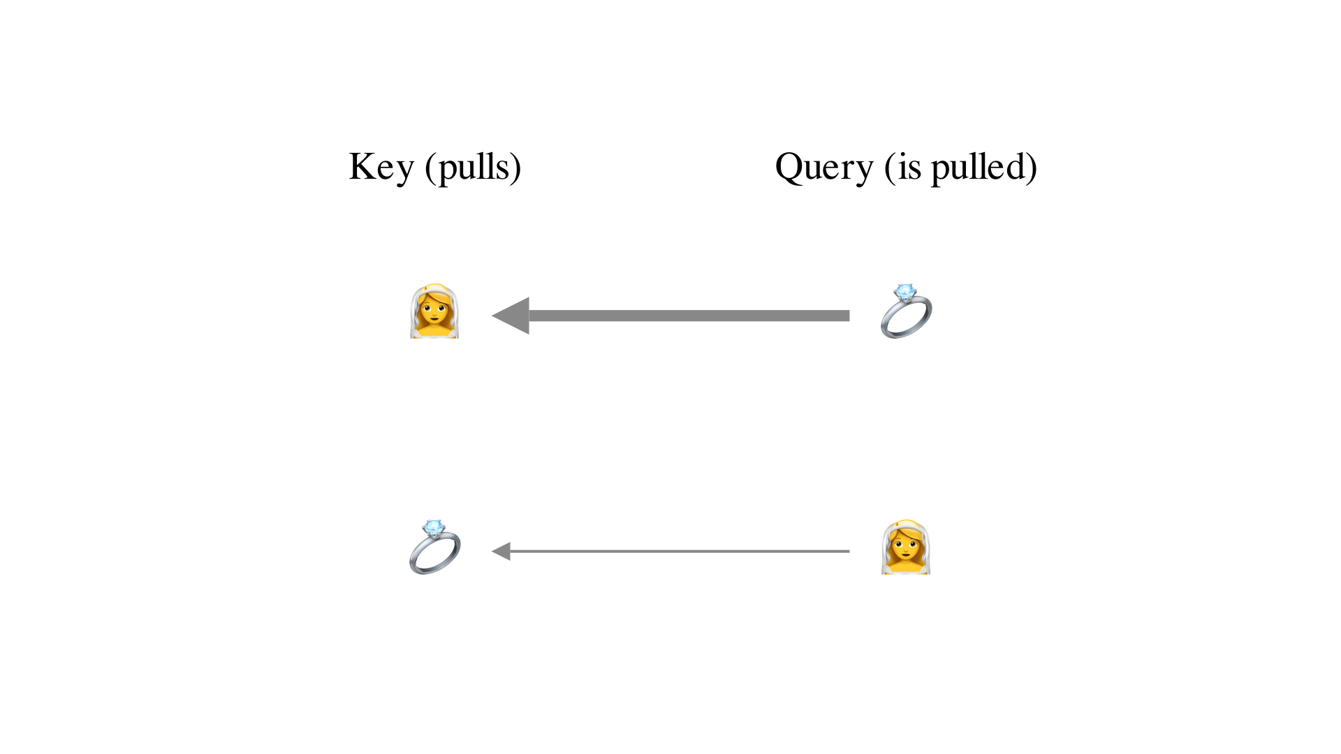
Let's introduce some vocabulary to describe this. We will call the word that is being pulled the query, and the word that pulls the key. In our "bride" and "ring" example, we want this:

• When "bride" is the key and "ring" is the query — that is when "bride" pulls "ring" — we want a strong pulling force.
• But when "ring" is the key and "bride" is the query — that is when "ring" pulls "bride" — we want a weaker pulling force.

Our desired asymmetric pulling forces.

How do we create these asymmetric forces? We know that the only thing that determines the pulling force is the similarity between the embedding vectors. So, we have to make the similarity different depending on which vector is acting as the query and which is acting as the key. What if we applied one transformation to the queries and another one to the keys? Let's have a look.

We'll start by placing "bride" and "ring" in a shared 2D embedding space. Then, we’ll make a copy: the left will represent the key space, and the right will represent the query space. When we calculate the force that "bride" pulls "ring", we will use the "bride" vector from key space (remember keys pull) and the "ring" vector from the query space (queries are pulled). And when we compute the force that "ring" pulls "bride", we use the "ring" vector from the key space and the "bride" vector from the query space. Since these spaces are currently identical, the two pairs of vectors are equally similar.

Here’s where things get interesting: by applying different transformations to the key and query spaces, we can make their similarity asymmetric. Let's apply a transformation squooshing the x-axis to the key space and one squooshing the y-axis to the query space. Now, when we take the "bride" vector from the key space and the "ring" vector from the query space, we see that they are very similar. So, they have a high dot product. This means that "bride" will exert a strong pulling force on "ring". But when we take the "ring" vector from the key space and the "bride" vector from the query space, we get two vectors that are not as similar. They have a lower dot product. So, the pulling force that "ring" exerts on "bride" is much weaker.

Let's now apply this to our running example of how "apple" gets pulled in the phrase "I ate a banana and an apple". We compute the dot product between the query vector for "apple" (the word being pulled) and the key vectors for every other word (the ones doing the pulling). We will denote queries by $q$ and keys by $k$, and the matrices used to compute them as $W_Q$ and $W_K$, respectively.

We then apply softmax to these dot products to get the attention scores — the coefficients used in the weighted average that produces the new vector for "apple".

Keys, Queries, and Values

We’ve now introduced three transformations applied to each embedding vector — producing the keys, queries, and values:

• $\vec{k} = W_K \vec{x}$
• $\vec{q} = W_Q \vec{x}$
• $\vec{v} = W_V \vec{x}$

Let's briefly recap the purpose of each before we look at how this affects our application of attention to the whole phrase.

Keys and queries define spaces that optimize how we measure similarity. They can highlight features that matter for similarity, suppress irrelevant ones, and even combine features in meaningful ways. All in a way to create the most optimal spaces to compute how strongly each word should pull the others. Importantly, having two separate transformations allows for asymmetric pull. In our linear combination that computes the updated vector, the keys and queries produce the coefficients — the attention scores.

Values define the space in which we move the embeddings. They emphasize features that help distinguish between different meanings — enabling attention to update vectors in contextually meaningful ways. Given the weights computed by the keys and queries, we combine value vectors to compute the updated vector for a word.

Just like the weights in our classifier, the matrices $W_K$, $W_Q$, and $W_V$ are learned — adjusted during training on massive amounts of text — to optimize the behavior of attention.

The Whole Phrase — with Keys, Queries, and Values

Recall that we stacked all the embedding vectors for the phrase as rows in a matrix, $X$. To generate the keys, queries, and values, we multiply $X$ by the three learned matrices $W_K$, $W_Q$, and $W_V$. We will call these new matrices $K$, $Q$, and $V$.

• $K = X W_K$
• $Q = X W_Q$
• $V = X W_V$

Next, we compute the dot product between every query and every key. This is done efficiently via matrix multiplication: $QK^T$. Just as before, the next step is to apply softmax to each row: $\text{softmax}(QK^T)$. Finally, we use these weights to compute a weighted average of the values — one row at a time — which gives us the updated vectors. This can be written as $\text{softmax}(QK^T)V$.

Let’s walk through this visually using the same table format from before. First, we apply our transformations to get keys and queries. Next, we take the dot product between each pair of keys and queries and apply softmax to each row. We now have the coefficients for the weighted average that computes the updated embedding vectors. To get the vectors for the weighted average, we take a copy of our original vectors and transform them into values.

Multiple Key, Query, and Value Spaces

So far, we've seen one set of transformed spaces: one for keys, one for queries, and one for values. Take the value space, for example. It was made to separate different meanings of words, such as the two meanings of “apple.” In other words, it captures the semantics of a word. But semantics is not the only way words influence each other, and thus not the only thing we should take into account when updating the embedding of a word.

We would like to be able to simultaneously consider many different linguistic features. In addition to semantics, we also want to consider something like grammatical relations. For example, we want to capture how adjectives modify nouns — like distinguishing a red apple from a green one.

How can we consider multiple linguistic features at once? Instead of using just one value space, we will use multiple. Each space will capture a different linguistic pattern and update the embeddings in its own way.

Let's call the value space we discussed earlier the semantic space. It is tuned to reflect how words are used in context. Take the phrase "I ate a banana and a red apple". The semantic space works just as before: it gives the most effect of pulling "apple" towards "banana", separating it from the technology brand.

Next, let's develop a grammatical relations space. In this space, we want "apple" to be shifted in a way such that it embodies a red apple more than any other color of apple.

We have described two different value spaces. Let's call the weight matrix for the semantic transformation $W_V^{(0)}$ and for the grammatical relations transformation $W_V^{(1)}$.

Similarly to how we developed these, we will find it useful to have two sets of key and query transformations as well: $W_K^{(0)}$ and $W_K^{(1)}$, and $W_Q^{(0)}$ and $W_Q^{(1)}$.

We will use the same index notation for the two sets of key, query, and value matrices:

• $K^{(i)} = X W_K^{(i)}$
• $Q^{(i)} = X W_Q^{(i)}$
• $V^{(i)} = X W_V^{(i)}$

This gives us two formulas for attention — that is for computing the updated vectors:

• $\text{softmax}(Q^{(0)}(K^{(0)})^T)V^{(0)}$
• $\text{softmax}(Q^{(1)}(K^{(1)})^T)V^{(1)}$

This is called two heads of attention.

But we now have two sets of updated embedding vectors: one from each head. We still want only one set of embedding vectors. How do we combine them into one?

We could simply average the two results. But by now, we recognize a better option: let the model learn how to combine them. In some contexts, semantics may be more important, while in others, grammatical relations are more important.

Let's call the two matrices of updated row vectors $\text{head}^{(0)}$ and $\text{head}^{(1)}$. If we place them side-by-side in one big matrix $O$, we can then multiply this matrix by a learned weight matrix $W_O$ to project $O$ back down to the original embedding size. This way, the model can not only learn to emphasize and deemphasize the two spaces, but it can also combine and reorient the vectors.

We can extend this beyond two heads. Modern models use many more heads. For example, DeepSeek-V3, a top-performing open-source model, uses 128 attention heads according to the technical report. (Although it has a very clever optimization that essentially gives the effect of 128 heads while using less memory and compute. This Welch Labs video provides an excellent explanation.)

Using multiple heads in attention is called multi-head attention and it was one of the major breakthroughs in the famous 2017 paper Attention Is All You Need.

Increasing the Dimensionality

Let’s make one final generalization. To motivate the example above, we added colors to our embedding space. This doesn't make a whole lot of sense. Previously, we said the axes might correspond to ideas like fruitiness and techiness. So where does color fit in? It doesn’t — at least not in a 2D space. What we really want is a third dimension, one that captures color. More generally, we want each concept we care about to have its own direction in space.

Modern models like DeepSeek-V3 use enormous embedding dimensions — 7168, in this case. With that many dimensions, you can begin to see why attention is so powerful: the model has thousands of directions to represent and reason over different concepts.

But it gets even better. In an $N$-dimensional space, you can fit at most $N$ mutually independent (orthogonal) directions — that is, vectors that are exactly $90^\circ$ apart. But it turns out that if we loosen that requirement just a little — allowing vectors to be nearly orthogonal (say, between $89^\circ$ and $91^\circ$ apart) — we can fit exponentially more.

It follows from a mathematical lemma, called the Johnson–Lindenstrauss lemma, that the number of approximately independent directions you can fit is about $e^{\epsilon \cdot N}$ for small $\epsilon$. So, with 7168 dimensions, it’s not just 7168 concepts — it’s on the order of $e^{7168}$. That’s a number with over 3000 digits (!!). In other words, high-dimensional spaces are incredibly expressive.

Finally, let's revisit our formula for attention:

As we increase the dimension of the keys and queries, their dot products tend to grow in magnitude — simply because they include more terms. When passed into softmax, these large values make the output too peaky — with one score close to 1 and all others near 0 — which can make the model harder to train.

To fix this, we scale the dot products by dividing by $\sqrt{d_k}$, where $d_k$ is the dimensionality of the keys and queries. This keeps the softmax outputs at a manageable scale. This gives us the final formula for attention:

Because of the scaling factor $\frac{1}{\sqrt{d_k}}$, this is commonly referred to as scaled dot product attention.

And there it is — the exact formula introduced in the landmark 2017 paper Attention Is All You Need.

Some Things We Didn't Cover

While we have covered a lot, there are plenty of things we have skipped over:

• Tokenization: We've assumed that each word gets its own embedding vector. That's not quite true. In practice, models break the input into tokens. Common words like "apple" or "banana" might be a single token, but longer or rarer words — like "unbelievable" — may be split into multiple tokens (e.g., "un", "believ", and "able"). This lets the model handle rare or unknown words and share knowledge across similar ones (like "runner" and "runners").
• How embeddings are learned: The way we described embeddings, it seems like they are manually crafted. In reality, they're actually learned during training. How this happens — and what kinds of structure the learned embeddings contain — is a fascinating topic of its own.
• Positional encodings: Attention is permutation-invariant — meaning the word order doesn’t matter. Without additional information, the model sees “the dog chased the cat” the same as “the cat chased the dog.” To fix this, we add positional encodings to the embeddings, so the model knows where each token appears in the sequence.
• Masking: Especially during training, we don’t want the model to cheat by looking ahead. When predicting the next word, it shouldn’t be able to see future words in the sequence. To prevent this, we mask out future tokens — setting their attention scores to zero — so the model only attends to previous and current tokens.
• How attention is trained: We've repeatedly said that the weights are learned, but we haven't said how. Like most modern machine learning models, attention-based models are trained with gradient descent and backpropagation. If you understand those techniques from simpler models, the same ideas apply here too.
• Feedforward layers in Transformers: Attention is often used in a broader architecture called the Transformer. In Transformers, attention layers alternate with feedforward layers — standard neural networks that help refine the representation at each step. We haven't touched on how feedforward layers contribute to generating better text.
• Optimizations to attention: Attention is computationally expensive. It scales quadratically with input length. To make it faster and more memory efficient, several optimizations have been developed. These include: multi-query attention (MQA), grouped-query attention (GQA), and multi-head latent attention (MLA).

Acknowledgments

The idea of interpreting attention as words pulling words was first introduced to me through this video by Serrano Academy. Some of the examples used in this post are adapted from Serrano Academy’s excellent videos on the topic.

Appendix: All Formulas and Shapes

It may be helpful to collect all the formulas and matrix shapes in one place. We'll do that here.